Asymptotics#
广大如法界,究竟如虛空
Asymptotic theory is a set of mathematical tools that invoke limits to simplify our understanding of the behavior of statistics.
Modes of Convergence#
Let \(x_{1},x_{2},\ldots\) be a (countably) infinite sequence of non-random variables. Convergence of this non-random sequence means that for any \(\varepsilon>0\), there exists an \(N\left(\varepsilon\right)\) such that for all \(n>N\left(\varepsilon\right)\), we have \(\left|x_{n}-x\right|<\varepsilon.\)
Example
\(x_{1,n} = 1 + 1/n\) is a sequence, with limit 1. \(x_{2,n} = - \exp(-n)\) is another sequence, with limit 0.
We learned limits of deterministic sequences in high school. Now, we discuss convergence of a sequence of random variables. Since a random variable is “random”, we must be clear what convergence means. Several modes of convergence are widely used.
We say a sequence of random variables \(\left(x_{n}\right)\) converges in probability to \(x\), where \(x\) can be either a random variable or a non-random constant, if for any \(\varepsilon>0\) the probability
as \(n\to\infty\). We write \(x_{n}\stackrel{p}{\to}x\) or \(\mathrm{plim}_{n\to\infty}x_{n}=x\).
A sequence of random variables \(\left(x_{n}\right)\) converges in squared-mean to \(x\), where \(x\) can be either a random variable or a non-random constant, if \(E\left[\left(x_{n}-x\right)^{2}\right]\to0.\) It is denoted as \(x_{n}\stackrel{m.s.}{\to}x\).
In these definitions either \(P\left\{ \left|x_{n}-x\right|>\varepsilon\right\}\) or \(E\left[\left(x_{n}-x\right)^{2}\right]\) is a non-random quantity, and it thus converges to 0 as a non-random sequence under the standard meaning of “\(\to\)”.
Squared-mean convergence is stronger than convergence in probability. That is, \(x_{n}\stackrel{m.s.}{\to}x\) implies \(x_{n}\stackrel{p}{\to}x\) but the converse is untrue. Here is an example.
Example
\((x_{n})\) is a sequence of binary random variables: \(x_{n}=\sqrt{n}\) with probability \(1/n\), and \(x_{n}=0\) with probability \(1-1/n\). Then \(x_{n}\stackrel{p}{\to}0\) but \(x_{n}\stackrel{m.s.}{\nrightarrow}0\). To verify these claims, notice that for any \(\varepsilon>0\), we have \(P\left(\left|x_{n}-0\right|<\varepsilon\right)=P\left(x_{n}=0\right)=1-1/n\rightarrow1\) and thereby \(x_{n}\stackrel{p}{\to}0\). On the other hand, \(E\left[\left(x_{n}-0\right)^{2}\right]=n\cdot1/n+0\cdot(1-1/n)=1\nrightarrow0,\) so \(x_{n}\stackrel{m.s.}{\nrightarrow}0\).
This example highlights the difference between the two modes of convergence. Convergence in probability does not take account extreme events with small probability. Squared-mean convergence, instead, deals with the average over the entire probability space. If a random variable can take a wild value, with small probability though, it may blow away the squared-mean convergence. On the contrary, such irregularity does not destroy convergence in probability.
Both convergence in probability and squared-mean convergence are about convergence of random variables to a target random variable or constant. That is, the distribution of \((x_{n}-x)\) is concentrated around 0 as \(n\to\infty\). Convergence in distribution is, however, about the convergence of CDF, instead of the random variable.
Let \(F_{n}\left(\cdot\right)\) be the CDF of \(x_{n}\) and \(F\left(\cdot\right)\) be the CDF of \(x\). We say a sequence of random variables \(\left(x_{n}\right)\) converges in distribution to a random variable \(x\) if \(F_{n}\left(a\right)\to F\left(a\right)\) as \(n\to\infty\) at each point \(a\in\mathbb{R}\) where \(F\left(\cdot\right)\) is continuous. We write \(x_{n}\stackrel{d}{\to}x\).
Convergence in distribution is the weakest mode. If \(x_{n}\stackrel{p}{\to}x\), then \(x_{n}\stackrel{d}{\to}x\). The converse is untrue in general, unless \(x\) is a non-random constant (A constant \(x\) can be viewed as a degenerate random variables.)
Example
Let \(x\sim N\left(0,1\right)\). If \(x_{n}=x+1/n\), then \(x_{n}\stackrel{p}{\to}x\) and of course \(x_{n}\stackrel{d}{\to}x\). However, if \(x_{n}=-x+1/n\), or \(x_{n}=y+1/n\) where \(y\sim N\left(0,1\right)\) is independent of \(x\), then \(x_{n}\stackrel{d}{\to}x\) but \(x_{n}\stackrel{p}{\nrightarrow}x\).
Example
\((x_{n})\) is a sequence of binary random variables: \(x_{n}=n\) with probability \(1/\sqrt{n}\), and \(x_{n}=0\) with probability \(1-1/\sqrt{n}\). Then \(x_{n}\stackrel{d}{\to}x=0.\) Because
Let \(F \left(a\right)=\begin{cases} 0, & a<0\\ 1 & a\geq0 \end{cases}\). It is easy to verify that \(F_{n}\left(a\right)\) converges to \(F\left(a\right)\) pointwisely on each point in \(\mathbb{R}\backslash \{0\}\), where \(F\left(a\right)\) is continuous.
So far we have talked about convergence of scalar variables. These three modes of convergence can be easily generalized to finite-dimensional random vectors.
Law of Large Numbers#
Law of large numbers (LLN) is a collection of statements about convergence in probability of the sample average to its population counterpart. The basic form of LLN is:
as \(n\to\infty\). Various versions of LLN work under different assumptions about moment restrictions and/or dependence of the underlying random variables.
Chebyshev LLN#
We illustrate LLN by the simple example of Chebyshev LLN. It utilizes the Chebyshev inequality.
The Chebyshev inequality is a special case of the Markov inequality.
Markov inequality: If a random variable \(x\) has a finite \(r\)-th absolute moment \(E\left[\left|x\right|^{r}\right]<\infty\) for some \(r\ge1\), then we have \(P\left\{ \left|x\right|>\varepsilon\right\} \leq E\left[\left|x\right|^{r}\right]/\varepsilon^{r}\) any constant \(\varepsilon>0\).
Rearrange the above inequality and we obtain the Markov inequality.
Let the partial sum \(S_{n}=\sum_{i=1}^{n}x_{i}\) where \(x_i\) are independently and identically distributed (i.i.d.). Let \(\mu=E\left[x_{1}\right]\) and \(\sigma^{2}=\mathrm{var}\left[x_{1}\right]\). We apply the Chebyshev inequality to the sample mean \(y_{n}:=\bar{x}-\mu=n^{-1}\left(S_{n}-E\left[S_{n}\right]\right)\). We have
This result gives the Chebyshev LLN:
Chebyshev LLN: If \(\left(x_{1},\ldots,x_{n}\right)\) is a sample of iid observations with \(E\left[x_{1}\right]=\mu\) and \(\sigma^{2}=\mathrm{var}\left[x_{1}\right]<\infty\), then \(\frac{1}{n}\sum_{i=1}^{n}x_{i}\stackrel{p}{\to}\mu.\)
Another useful LLN is the Kolmogorov LLN. Since its derivation requires more advanced knowledge of probability theory, we state the result without proof.
Kolmogorov LLN: If \(\left(x_{1},\ldots,x_{n}\right)\) is a sample of iid observations and \(E\left[x_{1}\right]=\mu\) exists, then \(\frac{1}{n}\sum_{i=1}^{n}x_{i}\stackrel{p}{\to}\mu\).
Compared with the Chebyshev LLN, the Kolmogorov LLN only requires the existence of the population mean, but not any higher moments. On the other hand, iid is essential for the Kolmogorov LLN.
Example
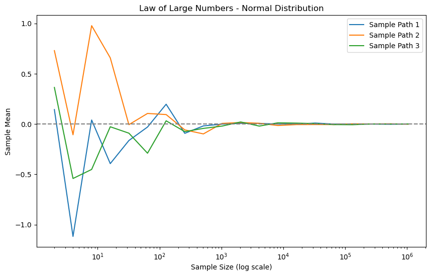
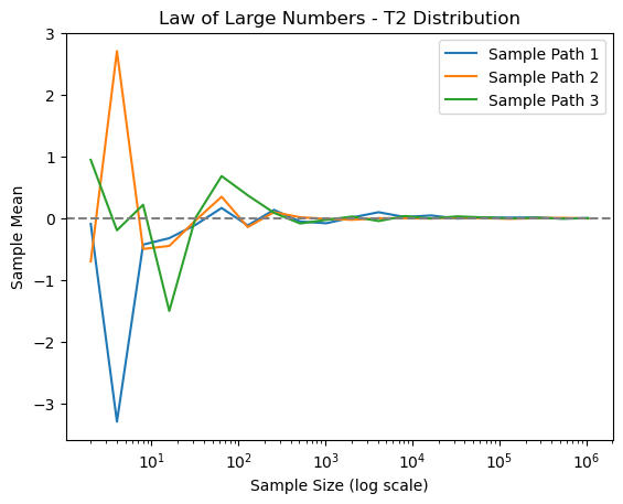
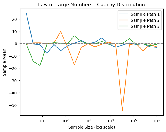
This script demonstrates LLN along with the underlying assumptions. Consider three distributions: standard normal \(N\left(0,1\right)\), \(t\left(2\right)\) (zero mean, infinite variance), and the Cauchy distribution (no moments exist). We plot paths of the sample average with \(n=2^{1},2^{2},\ldots,2^{20}\). We will see that the sample averages of \(N\left(0,1\right)\) and \(t\left(2\right)\) converge, but that of the Cauchy distribution does not.
import numpy as np
from scipy.stats import norm, t, cauchy
import pandas as pd
np.random.seed(45)
def sample_mean(n, distribution):
    """
    This function calculates the sample mean for a given distribution.

    Parameters:
    - n: Number of samples.
    - distribution: Type of distribution ('normal', 't2', or 'cauchy').

    Returns:
    - The mean of the generated samples.
    """
    if distribution == "normal":
        y = norm.rvs(size=n)
    elif distribution == "t2":
        y = t.rvs(df=2, size=n)
    elif distribution == "cauchy":
        y = cauchy.rvs(size=n)
    else:
        raise ValueError("Unsupported distribution")

    return np.mean(y)
This function plots the sample mean over the path of geometrically increasing sample sizes.
import numpy as np
import matplotlib.pyplot as plt
from scipy.stats import norm, t, cauchy

def LLN_plot(distribution):
    NN = 2**np.arange(1, 21)  # Sample sizes
    ybar = np.zeros((len(NN), 3))
    for rr in range(3):
        for ii, n in enumerate(NN):
            ybar[ii, rr] = sample_mean(n, distribution)

    for i in range(3):
        plt.plot(NN, ybar[:, i], label=f'Sample Path {i+1}')
    plt.axhline(0, color='grey', linestyle='--')
    plt.xscale('log')
    plt.xlabel('Sample Size (log scale)')
    plt.ylabel('Sample Mean')
    plt.title(f'Law of Large Numbers - {distribution.capitalize()} Distribution')
    plt.legend()
    plt.show()

# np.random.seed(2024-7-25) # Set seed for reproducibility


# Plotting
plt.figure(figsize=(10, 6))
LLN_plot("normal")
LLN_plot("t2")
LLN_plot("cauchy")
Central Limit Theorem#
The central limit theorem (CLT) is a collection of statements about the convergence in distribution to a stable distribution. The limiting distribution is usually the Gaussian distribution.
Various versions of CLT work under different assumptions about the random variables. Lindeberg-Levy CLT is the simplest version.
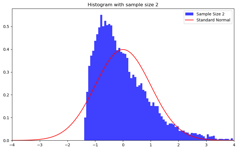
If the sample \(\left(x_{1},\ldots,x_{n}\right)\) is iid, \(E\left[x_{1}\right]=0\) and \(\mathrm{var}\left[x_{1}\right]=\sigma^{2}<\infty\), then \(\frac{1}{\sqrt{n}}\sum_{i=1}^{n}x_{i}\stackrel{d}{\to}N\left(0,\sigma^{2}\right)\).
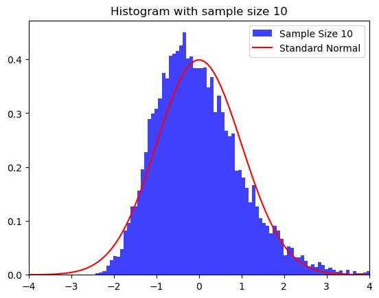
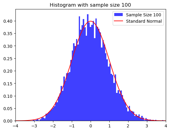
This is a simulated example.
Example
\(\chi^2(2)\) distribution with sample sizes \(n=2\), \(10\), and \(100\).
import numpy as np
import matplotlib.pyplot as plt
from scipy.stats import norm, chi2

def Z_fun(n, distribution):
    if distribution == "normal":
        z = np.sqrt(n) * np.mean(np.random.normal(size=n))
    elif distribution == "chisq2":
        df = 2
        x = np.random.chisquare(df, n)
        z = np.sqrt(n) * (np.mean(x) - df) / np.sqrt(2*df)
    return z

def CLT_plot(n, distribution):
    Rep = 10000
    ZZ = np.array([Z_fun(n, distribution) for _ in range(Rep)])

    xbase = np.linspace(-4.0, 4.0, 100)
    plt.hist(ZZ, bins=100, density=True, alpha=0.75,
             label=f'Sample Size {n}', color='blue')
    plt.plot(xbase, norm.pdf(xbase), color='red', label='Standard Normal')
    plt.xlim([np.min(xbase), np.max(xbase)])
    plt.title(f"Histogram with sample size {n}")
    plt.legend()
    plt.show()

# Plotting
plt.figure(figsize=(10, 6))
CLT_plot(2, "chisq2")
CLT_plot(10, "chisq2")
CLT_plot(100, "chisq2")
Tools for Transformations#
Continuous mapping theorem 1: If \(y_{n}\stackrel{p}{\to}a\) and \(f\left(\cdot\right)\) is continuous at \(a\), then \(f\left(y_{n}\right)\stackrel{p}{\to}f\left(a\right)\).
Continuous mapping theorem 2: If \(z_{n}\stackrel{d}{\to} z\) and \(f\left(\cdot\right)\) is continuous almost surely on the support of \(z\), then \(f\left(z_{n}\right)\stackrel{d}{\to}f\left(z\right)\).
Slutsky’s theorem: If \(y_{n}\stackrel{p}{\to}a\) and \(z_{n}\stackrel{d}{\to}z\) and, then
\(z_{n}+y_{n}\stackrel{d}{\to}z+a\)
\(z_{n}y_{n}\stackrel{d}{\to}az\)
\(z_{n}/y_{n}\stackrel{d}{\to}z/a\) if \(a\neq0\).
Slutsky’s theorem consists of special cases of the continuous mapping theorem 2.
Case Study#
Price-Weighted Stock Indexes
In the realm of financial markets, stock indexes serve as vital barometers, distilling the complex interplay of thousands of individual securities into a single, digestible metric. Among these, price-weighted indexes such as the Dow Jones Industrial Average (DJIA) and the Nikkei 225 stand out for their simplicity. The DJIA, comprising 30 blue-chip companies listed on U.S. exchanges, and the Nikkei 225, tracking 225 prominent stocks on the Tokyo Stock Exchange, both calculate their values by essentially averaging the prices of their constituent stocks (adjusted for factors like splits and changes).
Individual stock prices are influenced by corporate earnings, investor sentiment, geopolitical events, etc. Each stock’s price is inherently prone to idiosyncratic risks. However, when aggregated into an index, these prices form a larger sample. The LLN suggests that the average of these prices should stabilize around an expected value reflective of broader market conditions.
In essence, price-weighted indexes operationalize the LLN by treating stock prices as random variables whose mean reveals underlying truths. This averaging process not only measures market health but also informs economic policy. Central banks like the Federal Reserve or Bank of Japan closely monitor these indexes. Stock prices, in aggregate, incorporate forward-looking information about corporate profitability, which ties into economic fundamentals like GDP growth, employment, and inflation. Price-weighted stock indexes are practical manifestations of LLN, where the aggregation of individual stock prices yields a cross-sectionally stable average. In the multitude of prices, the truth emerges, steady and revealing.
As a final note, in Asia’s premier financial center, Hong Kong’s flagship Hang Seng Index (HSI) differs from price-weighted indexes. HSI weights companies based on the market value of their publicly tradable shares. Similarly, in Mainland China the Shanghai Composite (SSE) and CSI300 are also weighted indices.
投资有风险,入市需谨慎。以下个人观点,不构成投资建议。
How are these indices related to our daily life? For these major stock indices, there are exchange-traded funds (ETFs) tradable like individual stocks. For example, IYY:NYSE is based on DJIA, and 2833:HK is based on HSI. They make a well diversified portfolio with risks lower than individual stocks, thanks to LLN. They are reasonable choices of passive investment for people who do not have confidence about their stock-picking skills.