Probability#
玄之又玄,众妙之门
Probability theory talks about the construction and implications of probability models. For example, given a probability distribution, what are the mean and variance? What is the distribution of a transformed random variable? In computer simulations, probability theory tells us what will happen to the generated realizations, in particular when the experiments can be repeated as many times as the researcher wishes. This is a real-world analogue of the frequentist’s interpretation of probability.
Probability Space#
A sample space \(\Omega\) is a collection of all possible outcomes. It is a set of things.
An event \(A\) is a subset of \(\Omega\). It is something of interest on the sample space.
A \(\sigma\)-field is a complete set of events that include all countable unions, intersections, and differences. It is a well-organized structure built on the sample space.
A probability measure satisfies
(positiveness) \(P\left(A\right)\geq0\) for all events;
(countable additivity) If \(A_{i}\) are mutually disjoint for \(i\in\mathbb{N}\), then \(P\left(\bigcup_{i\in\mathbb{N}}A_{i}\right)=\sum_{i\in\mathbb{N}} P \left(A_{i}\right).\)
\(P(\Omega) = 1\).
The above construction gives a mathematically well-defined probability measure, but we have not yet answered “How to assign the probability?”
There are two major schools of thinking on probability assignment. One is the frequentist, who considers probability as the average chance of occurrence if a large number of experiments are carried out. The other is the Bayesian, who deems probability as a subjective brief. The principles of these two schools are largely incompatible, while each school has peculiar pros and cons under different real-world contexts.
Questions for AI
Why do we need “measure theory” to define probability?
What is the Vitali set?
Random Variable#
A random variable maps an event to a real number. If the outcome is multivariate, we call it a random vector.
Data example
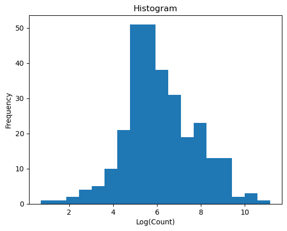
Data source: HK top 300 Youtubers. We look at the number of uploaded videos in these accounts.
import pandas as pd

# Reading the CSV file
d0 = pd.read_csv("HKTop300YouTubers.csv")
print(d0)
     rank                                           Youtuber subscribers  \
0       1                          Shadow MusicShadow Music    7,690,000
1       2                                  Emi WongEmi Wong    4,870,000
2       3                                iQIYI 爱奇艺iQIYI 爱奇艺    4,010,000
3       4  South China Morning PostSouth China Morning Post    2,650,000
4       5                                      GEM鄧紫棋GEM鄧紫棋    2,520,000
..    ...                                                ...         ...
295   296                          Jessica WongJessica Wong       69,000
296   297                                          昼与白鲸昼与白鲸       68,700
297   298                                        后宫冷婶儿后宫冷婶儿       68,600
298   299                              CatGirl貓女孩CatGirl貓女孩       68,200
299   300                                    男人EEETV男人EEETV       66,400

       video views video count          category  started
0    3,665,970,114       1,144    People & Blogs     2017
1      607,656,993         390    People & Blogs     2014
2    1,744,552,001       9,740  Film & Animation     2015
3    2,612,265,071      11,376   News & Politics     2007
4    1,752,111,944          77    People & Blogs     2019
..             ...         ...               ...      ...
295      3,008,911          80     Howto & Style     2014
296     18,950,918         156  Film & Animation     2020
297     43,142,355         323     Howto & Style     2020
298              0           0     Entertainment     2015
299      7,627,706         147            Comedy     2018

[300 rows x 7 columns]
# Remove NA and zeros by replacing zeros with NaN and then dropping rows with any NaN values
d0.replace(0, pd.NA, inplace=True)
d0.dropna(inplace=True)

# Select columns 3 to 5 (Python uses 0-based indexing, adjust accordingly)
d1 = d0.iloc[:, 2:5].copy()

# Rename columns
d1.columns = ["subs", "view", "count"] # "count" is the number of videos uploaded
print( d1 )
          subs           view   count
0    7,690,000  3,665,970,114   1,144
1    4,870,000    607,656,993     390
2    4,010,000  1,744,552,001   9,740
3    2,650,000  2,612,265,071  11,376
4    2,520,000  1,752,111,944      77
..         ...            ...     ...
295     69,000      3,008,911      80
296     68,700     18,950,918     156
297     68,600     43,142,355     323
298     68,200              0       0
299     66,400      7,627,706     147

[294 rows x 3 columns]
# convert string into numbers
for column in d1.columns:
    d1[column] = pd.to_numeric(d1[column].str.replace(',', ''), errors='coerce')

print(d1)
        subs        view  count
0    7690000  3665970114   1144
1    4870000   607656993    390
2    4010000  1744552001   9740
3    2650000  2612265071  11376
4    2520000  1752111944     77
..       ...         ...    ...
295    69000     3008911     80
296    68700    18950918    156
297    68600    43142355    323
298    68200           0      0
299    66400     7627706    147

[294 rows x 3 columns]
d1["count"]
0       1144
1        390
2       9740
3      11376
4         77
       ...
295       80
296      156
297      323
298        0
299      147
Name: count, Length: 294, dtype: int64
import numpy as np

# if any value is zero, remove the row
d1 = d1[(d1 != 0).all(axis=1)]
d1_log= np.log(d1)
import matplotlib.pyplot as plt

# Plotting histogram of the 'count' column after log transformation
plt.hist(d1_log['count'], bins='auto')  # 'auto' lets matplotlib decide the number of bins
plt.title('Histogram')
plt.xlabel('Log(Count)')
plt.ylabel('Frequency')
plt.show()
Distribution Function#
We go back to some terminologies we learned in an undergraduate probability course. A (cumulative) distribution function \(F:\mathbb{R}\mapsto [0,1]\) is defined as
It is often abbreviated as CDF, and it has the following properties.
\(\lim_{x\to-\infty}F\left(x\right)=0\),
\(\lim_{x\to\infty}F\left(x\right)=1\),
non-decreasing,
right-continuous \(\lim_{y\to x^{+}}F\left(y\right)=F\left(x\right).\)
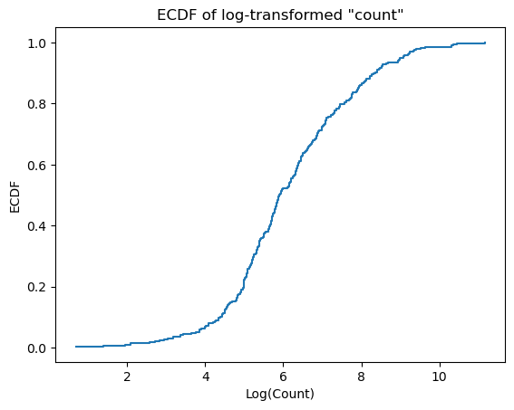
# Calculate the ECDF for the 'count' column
x = np.sort(d1_log['count'])
y = np.arange(1, len(x)+1) / len(x)

# Plot the ECDF as a step plot
plt.step(x, y, where='post')
plt.xlabel('Log(Count)')
plt.ylabel('ECDF')
plt.title('ECDF of log-transformed "count"')
plt.show()
The \(q\)-th quantile of a random variable is \(\min_{x\in \mathbb R} P(X \leq x) \geq q\).
d1_log['count'].quantile([0.25, 0.5, 0.75, 1.0])
0.25     5.087596
0.50     5.899897
0.75     7.107425
1.00    11.164587
Name: count, dtype: float64
For a continuous distribution, if its CDF is differentiable, then
is called the probability density function of \(X\), often abbreviated as PDF. It is easy to show that \(f\left(x\right)\geq0\), and by the Leibniz integral rule \(\int_{a}^{b}f\left(x\right)dx=F\left(b\right)-F\left(a\right)\).
For a discrete random variable, its CDF is obviously non-differentiable at any jump points. In this case, we define the probability mass function \(f(x) = F(x) - \lim_{y \to x^{-}} F(y)\).
We have learned many parametric distributions. A parametric distribution can be completely characterized by a few parameters.
Examples
Binomial distribution.
Poisson distribution.
Uniform distribution.
Normal distribution.
Its mean is \(\mu\) and variance \(\sigma^2\).
Log-normal distribution.
Its means is \(\exp(\mu + 0.5 \sigma^2)\) and variance \([\exp(\sigma^2 - 1)] \exp(2\mu+ \sigma^2)\).
\(\chi^{2}\), \(t\), and \(F\) distributions.
Example
scipy.stat has a rich collection of distributions.
from scipy.stats import norm

# Calculate the 97.5th percentile of the standard normal distribution
norm.ppf(0.975)
1.959963984540054
norm.cdf(0)
0.5
norm.pdf(0)
0.3989422804014327
# set a random seed for reproducibility
np.random.seed(42)
np.random.normal(size=3)
array([ 0.49671415, -0.1382643 , 0.64768854])
np.random.poisson(lam=50, size=3)
array([42, 52, 58])
Example 1
Below is a piece of code for demonstration.
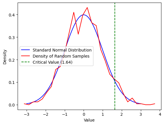
Plot the density of standard normal distribution over an equally spaced grid system.
Generate 1000 observations for \(N(0,1)\). Plot the histogram density, a nonparametric estimation of the density.
Calculate the 95th quantile and the empirical probability of observing a value greater than the 95th quantile. In population, this value is 5%. What is the number coming out of this experiment?
# Create x-axis from -3 to 3 with steps of 0.01
x_axis = np.arange(-3, 3, 0.01)

# Calculate the density of the standard normal distribution for x_axis
y = norm.pdf(x_axis)

# Plot the standard normal distribution density
plt.plot(x_axis, y, label='Standard Normal Distribution', color='blue')
plt.xlabel('Value')
plt.ylabel('Density')

# Generate 1000 random samples from a standard normal distribution
z = np.random.normal(size=1000)

# Calculate the density of the random samples and plot it
density = np.histogram(z, bins=30, density=True)
bin_centers = 0.5*(density[1][1:] + density[1][:-1])
plt.plot(bin_centers, density[0], color='red', label='Density of Random Samples')

# Calculate the critical value at the 95th percentile
crit = norm.ppf(0.95)

# Calculate the empirical rejection probability
empirical_rejection_probability = np.mean(z > crit)
print(f"The empirical rejection probability is {empirical_rejection_probability}")

# Add a vertical line for the critical value
plt.axvline(crit, color='green', linestyle='--', label=f'Critical Value ({crit:.2f})')

plt.legend()
plt.show()
The empirical rejection probability is 0.054
Integration#
In probability theory, an integral \(\int X\mathrm{d}P\) is called the expected value, or expectation, of \(X\). We often use the notation \(E\left[X\right]\), instead of \(\int X\mathrm{d}P\), for convenience.
The expectation is the average of a random variable, despite that we cannot foresee the realization of a random variable in a particular trial (otherwise there is no uncertainty). In the frequentist’s view, the expectation is the average outcome if we carry out a large number of independent trials.
If we know the probability mass function of a discrete random variable, its expectation is calculated as \(E\left[X\right]=\sum_{x}xP\left(X=x\right)\). If a continuous random variable has a PDF \(f(x)\), its expectation can be computed as \(E\left[X\right]=\int xf\left(x\right)\mathrm{d}x\).
np.mean( d1_log["count"] )
6.146389135729357
Here are some properties of the expectation.
\(E\left[X^{r}\right]\) is call the \(r\)-moment of \(X\). The mean of a random variable is the first moment \(\mu=E\left[X\right]\), and the second centered moment is called the variance \(\mathrm{var}\left[X\right]=E [(X-\mu)^{2}]\).
np.var(d1_log["count"])
2.6415986858999068
The third centered moment \(E\left[\left(X-\mu\right)^{3}\right]\), called skewness, is a measurement of the symmetry of a random variable, and the fourth centered moment \(E\left[\left(X-\mu\right)^{4}\right]\), called kurtosis, is a measurement of the tail thickness.
We call \(E\left[\left(X-\mu\right)^{3}\right]/\sigma^{3}\) the skewness coefficient, and \(E\left[\left(X-\mu\right)^{4}\right]/\sigma^{4}-3\) degree of excess. A normal distribution’s skewness and degree of excess are both zero.
Moments do not always exist. For example, the mean of the Cauchy distribution does not exist, and the variance of the \(t(2)\) distribution does not exist.
\(E[\cdot]\) is a linear operation. \(E[a X_1 + b X_2] = a E[X_1] + b E[X_2].\)
Jensen’s inequality is an important fact. A function \(\varphi(\cdot)\) is convex if \(\varphi( a x_1 + (1-a) x_2 ) \leq a \varphi(x_1) + (1-a) \varphi(x_2)\) for all \(x_1,x_2\) in the domain and \(a\in[0,1]\). For instance, \(x^2\) is a convex function. Jensen’s inequality says that if \(\varphi\left(\cdot\right)\) is a convex function, then
\[ \varphi\left(E\left[X\right]\right)\leq E\left[\varphi\left(X\right)\right]. \]Markov inequality is another simple but important fact. If \(E\left[\left|X\right|^{r}\right]\) exists, then
\[ P\left(\left|X\right|>\epsilon\right)\leq E\left[\left|X\right|^{r}\right]/\epsilon^{r} \]for all \(r\geq1\). Chebyshev inequality \(P\left(\left|X\right|>\epsilon\right)\leq E\left[X^{2}\right]/\epsilon^{2}\) is a special case of the Markov inequality when \(r=2\).
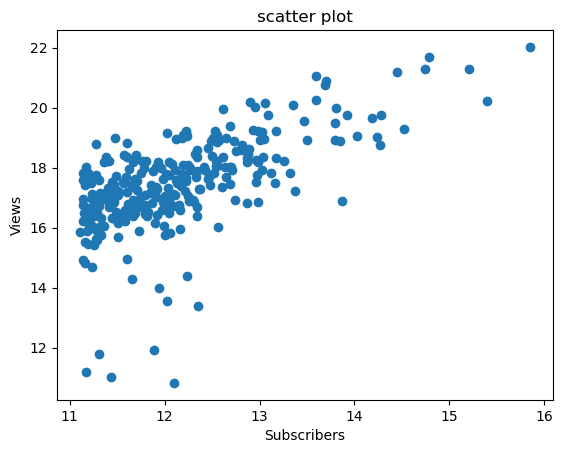
Multivariate Random Variable#
A bivariate random variable is a vector of two scalar random variables. More generally, a multivariate random variable has the joint CDF defined as
Joint PDF is defined similarly.
# Plotting 'subs' on the x-axis and 'view' on the y-axis
plt.plot(d1_log['subs'], d1_log['view'], marker='o', linestyle='None')
plt.xlabel('Subscribers')
plt.ylabel('Views')
plt.title('scatter plot')
plt.show()
It is illustrative to introduce the joint distribution, conditional distribution and marginal distribution in the simple bivariate case, and these definitions can be extended to multivariate distributions. Suppose a bivariate random variable \((X,Y)\) has a joint density \(f(\cdot,\cdot)\). The marginal density \(f\left(y\right)=\int f\left(x,y\right)dx\) integrates out the coordinate that is not interested. The conditional density can be written as \(f\left(y|x\right)=f\left(x,y\right)/f\left(x\right)\) for \(f(x) \neq 0\).
Bayes Theorem#
For two events \(A_1\) and \(A_2\), the conditional probability is
if \(P(A_2) \neq 0\). In this definition of conditional probability, \(A_2\) plays the role of the outcome space so that \(P(A_1 A_2)\) is standardized by the total mass \(P(A_2)\).
Since \(A_1\) and \(A_2\) are symmetric, we have \(P(A_1 A_2) = P(A_2|A_1)P(A_1)\). It implies
This formula is the well-known Bayes’ Theorem, which is a cornerstone of decision theory.
Example 2
\(A_1\) is the event “a student gets a CUHK Econ master offer”, and \(A_2\) is “his or her GPA higher than 3.5”. We are applying Bayes’ Theorem to compute the posterior probability \( P(A_1=1 \mid A_2) \)
Given the prior \(P(A_1=1) = 0.1\) (so \( P(A_1=0) = 0.9\)) and the likelihood \(P(A_2 \mid A_1=1) = 0.5\) and \(P(A_2 \mid A_1=0) = 0.05\), we compute the marginal probability \( P(A_2) \) using the law of total probability: \(P(A_2) = P(A_2 \mid A_1=1) \cdot P(A_1=1) + P(A_2 \mid A_1=0) \cdot P(A_1=0) = 0.5 \times 0.1 + 0.05 \times 0.9 = 0.095.\)
It follows that the posterior is \(P(A_1=1 \mid A_2) = \frac{0.5 \times 0.1}{0.095} = \frac{0.05}{0.095} \approx 0.5263.\) Notice the contrast: without knowing the GPA, the prior admission rate is only \(10\%\). The high GPA boosts it to \(52\%\).
Independence#
We say two events \(A_1\) and \(A_2\) are independent if \(P(A_1A_2) = P(A_1)P(A_2)\). If \(P(A_2) \neq 0\), it is equivalent to \(P(A_1 | A_2 ) = P(A_1)\). In words, knowing \(A_2\) does not change the probability of \(A_1\).
If \(X\) and \(Y\) are independent, then \(E[XY] = E[X]E[Y]\).
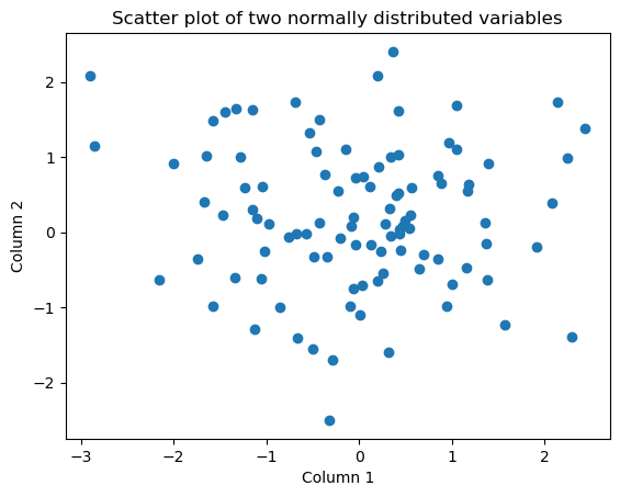
# Generate a 2-column matrix with 100 rows of random numbers from a standard normal distribution
Y = np.random.normal(size=(100, 2))

# Plot the first column against the second column
plt.scatter(Y[:, 0], Y[:, 1])
plt.xlabel('Column 1')
plt.ylabel('Column 2')
plt.title('Scatter plot of two normally distributed variables')
plt.show()
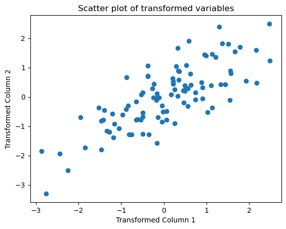
Y = np.random.normal(size=(100, 2))

# Apply the linear transformation
Y = np.dot(Y, np.array([[1, 0.5], [0.5, 1]]) )

# Plot the transformed data
plt.scatter(Y[:, 0], Y[:, 1])
plt.xlabel('Transformed Column 1')
plt.ylabel('Transformed Column 2')
plt.title('Scatter plot of transformed variables')
plt.show()
Law of Iterated Expectations#
In the bivariate case, if the conditional density exists, the conditional expectation can be computed as \(E\left[Y|X\right]=\int yf\left(y|X\right)dy\). The law of iterated expectation implies \(E\left[E\left[Y|X\right]\right]=E\left[Y\right]\).
# Add 'category' column from d0 to d1_log
d1_log['category'] = d0['category']

# Group by 'category' and calculate mean and count
dx = d1_log.groupby('category').agg(mean=('count', 'mean'), no=('count', 'size')).reset_index()

print(dx)
                 category      mean  no
0        Autos & Vehicles  7.516632   2
1                  Comedy  5.742748   8
2               Education  6.290369  10
3           Entertainment  6.342173  41
4        Film & Animation  5.976671  28
5                  Gaming  6.427200  28
6           Howto & Style  5.713592  31
7                   Music  5.914223  24
8         News & Politics  8.134565  22
9   Nonprofits & Activism  6.445720   1
10         People & Blogs  5.724408  68
11         Pets & Animals  6.188264   1
12   Science & Technology  6.083646   8
13                 Sports  6.140040   5
14        Travel & Events  5.483655  12
# Calculate weighted average over categories
weighted_avg = sum(dx['mean'] * (dx['no'] / len(d1_log)))
print(weighted_avg)
6.146389135729357
# Calculate and print overall average of 'count'
overall_avg = d1_log['count'].mean()
print(overall_avg)
6.146389135729357
Below are some properties of conditional expectations
\(E\left[E\left[Y|X_{1},X_{2}\right]|X_{1}\right]=E\left[Y|X_{1}\right];\)
\(E\left[E\left[Y|X_{1}\right]|X_{1},X_{2}\right]=E\left[Y|X_{1}\right];\)
\(E\left[h\left(X\right)Y|X\right]=h\left(X\right)E\left[Y|X\right].\)
Application
Regression is a technique that decomposes a random variable \(Y\) into two parts, a conditional mean and a residual. Write \(Y=E\left[Y|X\right]+\epsilon\), where \(\epsilon=Y-E\left[Y|X\right]\). Show that \(E[\epsilon] = 0\) and \(E[\epsilon E[Y|X] ] = 0\).
For the next lecture#
Save the following data files for the next lecture.
d1_log.to_csv('logYoutuber.csv', index=False)
# save a random subsmaple
d1_log_sub = d1_log.sample(n=100).to_csv('logYoutuber_sample.csv', index=False)
Story#

Two roads diverged in a yellow wood,
And sorry I could not travel both
We live in a world of uncertainty. About 20 years ago, students in China could select only one university as their first choice. It was a high-stakes gamble: success or failure carried lifelong consequences.
My Gaokao score fell short of my hopes, shattering my dreams of studying in Beijing or Shanghai. My options narrowed to Nanjing University (NJU) or Zhejiang University (ZJU). Back then, reliable information was scarce for would-be first-generation college-goers.
Zhejiang was my home province, and my high school routinely sent over 40 students to ZJU each year. Attending there wouldn’t earn me any bragging rights — it was expected. NJU, on the other hand, felt far more exotic. I had learned about it from a fellow small-town resident who had been admitted there and become a local legend, admired by every parent as an inspiring role model kid. For me, NJU was the dream school.
I managed to reach an NJU admissions representative by phone. After sharing my score and ranking, I asked which majors I might qualify for. He explained that my score was marginal. “You could try for geology,” he suggested half-heartedly. Geology wasn’t on my list of interests, but in my naivety, I thought it might not be so bad. I had read stories about Li Siguang, the geologist who pioneered oil exploration in China. Perhaps spending long stretches in the wilderness for fieldwork could even be romantic, I mused.
The decision loomed as a probability puzzle. I had two choices: ZJU or NJU. Each carried two possible consequences: success or failure. That yielded four scenarios, each with its own probability attached. Before submitting the piece of paper signalling my willingness, and before the cutoff scores were announced, I hung in suspense. What should I do? Shall I pursue my dream school, or play it safe?