Statistics#
形而上者谓之道,形而下者谓之器
Statistic theory goes the opposite way to probability theory. In reality what we observe is a sample of data, but we don’t know via what mechanism the data are generated. Statistics asks how can we infer the data generating process from the sample that we observe. For example, if we assume the sample comes from a normal distribution, what is the best way that we learn the population mean and variance? Do the data provide sufficient evidence that two samples are drawn from populations of the same means? Statistics uses the sample to compute some numbers, while the underlying probability model guides the interpretation of these numbers.
Example
This is a sample of 100 accounts from HK top 300 Youtubers which we randomly drew at the end of the previous lecture.
import pandas as pd
import numpy as np

# Reading the CSV file
d1_log_sub = pd.read_csv("logYoutuber_sample.csv")

# Checking the number of rows
n = d1_log_sub.shape[0]
print(n)
100
Point estimates
print(np.mean(d1_log_sub["count"]))
6.064122168009075
print(np.var(d1_log_sub["count"]))
2.494172970249846
We are interested in the sample mean, as it tells the location of the center in the probability weighted average, or population mean \(\mu = E[X_i]\). We are also interested in the sample variance, as it tells the scale of spread of the sample, or population variance \(\sigma^2 = var(X_i)\).
In this example, we can view the sample as a multinomial distribution with \(n\) outcomes at the observed realized points. Since each observation is drawn randomly and independently, everyone is equally important. Assigning equal probability \(1/n\) on each point naturally delivers the sample mean \(\hat{\mu} = \bar{X} = n^{-1} \sum_{i=1}^n X_i.\) Similarly, a widely used sample variance is computed as \(s^2 = (n-1)^{-1} \sum_{i=1}^n (X_i - \hat{\mu})^2\). More generally, for \(p>0\) the statistic \(n^{-1} \sum_{i=1}^n x_i^p\) is called the \(p\)-th sample moment, and \(n^{-1} \sum_{i=1}^n (X_i - \bar{X})^p\) is called the \(r\)-th centered moment.
Estimation methods#
Suppose that the data are generated from a parametric model. Statistical estimation is an “educated guess” of the unknown parameter from the observed data. A principle is an ideology about a proper way of estimation. Over the history of statistics, only a few principles are widely accepted. The two most popular methods are the method of moments and the maximum likelihood method.
Method of moments#
The method of moments expresses some moments as functions of these parameters. We use the sample moments to mimic the corresponding population moments. Then we invert the functions to back out the parameters.
Example
A normal distribution is completely characterized by \(\mu\) and \(\sigma^2\). The following two estimates are the method of moments estimates of the two parameters.
np.random.seed(43)

x = np.random.normal(size=20)

print(np.mean(x))
print(np.var(x))
-0.02302171273700368
0.9210986680193605
Example:
The \(t\) distribution has one parameter, its degree of freedom \(\nu\). The variance of \(t(\nu)\), if \(\nu >2\), is \(\sigma^2 = \nu / (\nu - 2)\). From the data, we estimate \(\hat{\sigma}^2\), and then solve \(\hat{\sigma}^2 = \nu / (\nu - 2)\) to get
Note: The population variance of \(t\) distribution is no smaller than 1.
Maximum likelihood#
The maximum likelihood estimation (MLE) looks for the value of the parameter that maximizes the log-likelihood. By the concavity of logarithm, the true parameter is the value that maximizes the expected likelihood function. In reality, we maximize its empirical version.
Consider a random sample drawn from a parametric distribution with density \(f\left(x;\theta\right)\), where \(x\) is either a scalar random variable or a random vector. A parametric distribution is completely characterized by a finite-dimensional parameter \(\theta\). We use the data to estimate \(\theta\).
The log-likelihood of observing the entire random sample \(\mathbf{X}=(X_1,X_2,\ldots,X_n)\) is
In reality the sample \(\mathbf{X}\) is given and for each \(\theta\in\Theta\) we can evaluate \(L_{n}\left(\theta;X\right)\). The maximum likelihood estimator is
This \(\widehat{\theta}_{MLE}\) makes observing \(X\) the “most likely” in the entire parametric space. A formal justification of MLE uses the terminology the Kullback-Leibler information criterion, which is a measurement of the “distance” or “divergence” between two distributions. This information criterion is maximized at the true parameter value.
Example
Consider the Gaussian model \(X_{i}\sim N\left(\mu, \sigma^2 \right)\), where \(\mu\) and \(\sigma\) are unknown parameters to be estimated. The likelihood of observing \(X_{i}\) is \(f\left(X_{i};\mu\right)=\frac{1}{\sqrt{2\pi}\sigma}\exp\left(-\frac{1}{2\sigma^2}\left(X_{i}-\mu\right)^{2}\right)\). The likelihood of observing the sample \(\mathbf{X}\) is
and the log-likelihood is
After some computation, we will find \(\hat{\mu}=n^{-1} \sum_{i=1}^n X_i\) and \(\hat{\sigma}^2 = n^{-1} \sum_{i=1}^n (X_i - \bar{X})^2\). Notice the denominator in the estimated variance here is \(n\), instead of \((n-1)\) as in \(s^2\). While \(s^2\) is an unbiased estimator for the variance, the MLE estimator is therefore biased for the variance.
Statistic Inference#
We are interesting in relating the statistic to the population. Suppose \(X_i\)’s are randomly drawn from a distribution, and we would like to learn the mean \(\mu: = E[X_i]\). The sample mean is a natural estimator for \(\mu\).
Interval estimation quantifies the uncertainty of the estimator. The most familiar formula might be
We will explain the rationale behind this formula.
import numpy as np

def CI(x):
    # x is a numpy array of random variables
    # nominal coverage probability is 95%
    n = len(x)
    mu = np.mean(x)
    sig = np.std(x)
    upper = mu + 1.96 / np.sqrt(n) * sig
    lower = mu - 1.96 / np.sqrt(n) * sig
    return {'lower': lower, 'upper': upper}
CI(d1_log_sub["count"])
{'lower': 5.754580331054653, 'upper': 6.373664004963498}
An interval estimator is constructed according to a sampling distribution. The sampling distribution is the distribution of a statistic.
Example
Sampling distributions. Under normal distribution
Assume \(X_i \sim N(\mu, \sigma^2)\) with a known variance. Then \(\bar{X} \sim N(\mu, \sigma^2 / n)\).
Assume \(X_i \sim N(\mu, \sigma^2)\) with a unknown variance. Then \(\frac{\bar{X} - \mu}{s} \sim t(n-1)\).
Assume \(X_i \sim (\mu, \sigma^2)\) with a finite variance. \(\sqrt{n} \frac{\bar{X} - \mu}{\sigma} \stackrel{d}{\rightarrow} N(0, 1)\). (to be discussed in asymptotic theory)
Example 3
In a simulation, we compute the empirical coverage probability of the formula of the confidence interval. The underlying data generating process is a Poisson distribution.
from scipy.stats import poisson

Rep = 1000
sample_size = 6
capture = np.zeros(Rep)
Bounds = np.zeros((Rep, 2))
mu = 2

for i in range(Rep):
    x = poisson.rvs(mu, size=sample_size)
    bounds = CI(x)
    capture[i] = ((bounds['lower'] <= mu) & (mu <= bounds['upper']))
    Bounds[i,] = [bounds['lower'], bounds['upper']]

print("The empirical coverage probability =", np.mean(capture))
The empirical coverage probability = 0.866
Coverage probability is the probability that the confidence interval captures the true value in repeated sampling. Here the confidence interval is random while the true value is fixed.
Example 4
Witness the confidence intervals from 25 replications.
import matplotlib.pyplot as plt

# Assuming Bounds is a numpy array with shape (Rep, 2) and contains the confidence intervals
Bounds25 = Bounds[:25, :]  # Extract the first 25 confidence intervals

plt.figure(figsize=(10, 6))
for i, (lower, upper) in enumerate(Bounds25, start=1):
    plt.plot([i, i], [lower, upper], marker='_', markersize=20, color='blue')  # Plot each confidence interval
plt.hlines(y=2, xmin=1, xmax=25, colors='red', linestyles='dashed', linewidth=2)  # True mean line

plt.xlim(1, 25)
plt.ylim(Bounds25.min(), Bounds25.max())
plt.xlabel('Sample Number')
plt.ylabel('Confidence Interval')
plt.title('Confidence Intervals for the First 25 Samples')
plt.show()
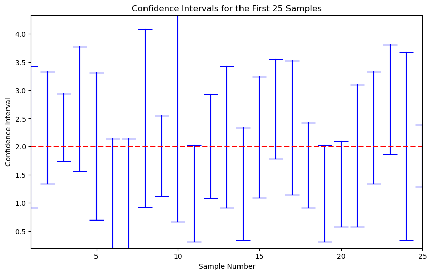
It is important to understand that the coverage probability is not the probability that the parameter falls into a fixed interval, which is the interpretation of the Bayesian credit interval. The latter requires different way for construction.
Hypothesis Testing#
A hypothesis is a statement about the parameter space \(\Theta\). Hypothesis testing checks whether the data support a null hypothesis \(\Theta_{0}\), which is a subset of \(\Theta\) of interest. Ideally the null hypothesis should be suggested by scientific theory. The alternative hypothesis \(\Theta_{1}=\Theta\backslash\Theta_{0}\) is the complement of \(\Theta_{0}\). Based on the observed evidence, hypothesis testing decides to accept or reject the null hypothesis. If the null hypothesis is rejected by the data, it implies that from the statistical perspective the data are incompatible with the proposed scientific theory.
Let \(\phi(\mathbf{X};\theta)\) be the decision function. It takes value “1” when \(\theta\) is rejected as a null hypothesis, and it takes value “0” otherwise. We define the power function \(\beta(\theta) = E[ \phi(\mathbf{X};\theta) ]\), which is the probability of rejecting a null hypothesis \(\theta\).
Actions, States and Consequences:
                |   accept $H_{0}$  |   reject $H_{0}$
  $H_{0}$ true  |  correct decision |    Type I error
  $H_{0}$ false |   Type II error   |  correct decision
The probability of committing Type I error is \(\beta\left(\theta\right)\) for some \(\theta\in\Theta_{0}\).
The probability of committing Type II error is \(1-\beta\left(\theta\right)\) for some \(\theta\in\Theta_{1}\).
The philosophy on hypothesis testing has been debated for a long time. At present the prevailing framework in statistics textbooks is the frequentist perspective. Frequentist views the parameter as fixed. They keep a conservative attitude about the Type I error: Only if overwhelming evidence is revealed shall a researcher reject the null. Under the principle of protecting the null hypothesis, a desirable test should have a small level. Conventionally we take \(\alpha=0.01,\) \(0.05\) or \(0.1\). We say a test is unbiased if
There can be many tests of correct size.
Remark 1
Let \(\mathbf{x} = (x_1, x_2, \ldots, x_n)\). A trivial test function \(\phi(\mathbf{x})=1\left\{ 0\leq U\leq\alpha\right\}\) for all \(\theta\in\Theta\), where \(U\) is a random variable from a uniform distribution on \(\left[0,1\right]\), has the correct size \(\alpha\) but no non-trivial power at the alternative. On the other extreme, the trivial test function \(\phi(\mathbf{x})=1\) for all \(\mathbf{x}\) enjoys the biggest power but suffers incorrect size.
Usually, we design a test by proposing a test statistic \(T_{n}\) and a corresponding critical value \(c_{1-\alpha}\). Given \(T_{n}\) and \(c_{1-\alpha}\), we write the test function as
To ensure such a \(\phi(\mathbf{x})\) has the correct size, we need to figure out the distribution of \(T_{n}\) under the null hypothesis (called the null distribution), and choose a critical value \(c_{1-\alpha}\) according to the null distribution where \(\alpha\) is the desirable size or level.
Another popular indicator for the compatibility between the data and the null hypothesis is the \(p\)-value:
In the above expression, \(T_{n}\left(\mathbf{x}\right)\) is the realized value of the test statistic \(T_{n}\), while \(T_{n}\left(\mathbf{X}\right)\) is the random variable generated by \(\mathbf{X}\) under the null \(\theta\in\Theta_{0}\). The interpretation of the \(p\)-value is tricky. \(p\)-value is the probability, when the null hypothesis is true, that we observe \(T_{n}(\mathbf{X})\) being greater than the realized \(T_{n}(\mathbf{x})\).
The \(p\)-value is not the probability that the null hypothesis is true. Under the frequentist perspective, the null hypothesis is either true or false, with certainty. The randomness of a test comes only from sampling, not from the hypothesis at all.
Connections#
Given the same sample and the underlying approach, hypothesis testing, confidence interval, and \(p\)-value are tightly connected. The followings are equivalent:
The hypothesized value is rejected by a test of size \(\alpha\);
The hypothesized value is excluded by the confidence interval of coverage probability \((1-\alpha)\);
Its \(p\)-value under the hypothesized value is smaller than \(\alpha\).
On the opposite side of the coin, the followings are the equivalent as well:
The hypothesized value is not rejected by a test of size \(\alpha\);
The hypothesized value is included by the confidence interval of coverage probability \((1-\alpha)\);
Its \(p\)-value under the hypothesized value is large than \(\alpha\).
The one-to-one mapping between the points in the confidence interval and the outcome of the test allows constructing the confidence interval by inverting the test. In words, if we collect all points that are not rejected by the test of size \(\alpha\), we obtain the confidence interval of coverage probability \((1-\alpha)\).
Revealing the population#
As in the previous lecture, we view the HK top 300 Youtubers as the population.
d1_log = pd.read_csv("logYoutuber.csv")

# Number of rows
N = d1_log.shape[0]
import numpy as np

print( np.mean(d1_log["count"]) )

print( np.var(d1_log["count"]) )

np.corrcoef(d1_log["count"], d1_log["view"])[0, 1]
6.146389135729357
2.6415986858999068
0.6086587545357828
print( np.mean(d1_log_sub["count"]) )

print( np.var(d1_log_sub["count"]) )

np.corrcoef(d1_log_sub["count"], d1_log_sub["view"])[0, 1]
6.064122168009075
2.494172970249846
0.4920793350404544
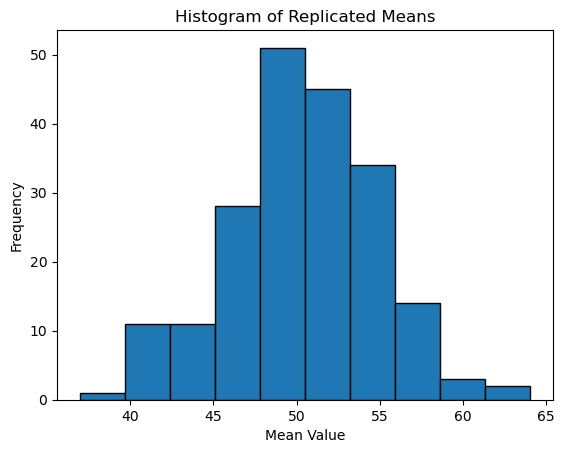
Random Sampling#
Each sample is random. It means that \(\hat{\mu}\) is a random variable across the potential samples. In this population the total number of outcomes is \(N=300\). For a sample of size \(n=100\), there are
possibilities for the sample mean. This is a number as large as all the atoms in the universe.
import numpy as np
import pandas as pd

# Assuming d1.log is a pandas DataFrame and 'count' is a column in that DataFrame
d1_log = pd.DataFrame({'count': np.random.randint(1, 100, size=1000)})  # Example data
N = len(d1_log['count'])
n = 50  # Example subsample size

def subsample_mean():
    indices = np.random.choice(range(N), n, replace=False)
    return d1_log['count'].iloc[indices].mean()

rep_means = np.array([subsample_mean() for _ in range(200)])

print(rep_means)
[56.72 50.16 48.98 54.38 46.78 45.94 51.02 56.7  52.72 51.8  49.22 53.42
 64.08 46.14 41.48 51.26 53.1  54.98 49.06 41.4  49.94 46.44 60.2  51.9
 56.22 46.3  43.32 49.5  46.3  48.94 52.12 58.44 48.3  51.94 43.66 46.18
 43.28 49.36 52.64 45.38 45.6  52.42 50.2  54.5  51.22 55.86 55.82 50.96
 46.62 41.96 51.46 48.22 56.34 44.22 40.9  52.42 48.28 57.78 50.96 55.24
 51.8  51.   51.6  57.26 51.8  46.76 51.08 46.16 55.56 54.92 49.9  48.46
 55.7  48.68 43.74 45.64 41.36 55.72 48.8  48.82 49.74 53.96 52.54 53.12
 45.48 48.88 52.82 51.68 44.2  55.38 50.02 49.96 45.02 48.84 49.84 48.22
 49.54 51.54 55.86 49.44 62.52 57.54 48.06 45.38 51.34 45.1  52.62 48.86
 51.98 42.18 48.26 48.84 51.   49.6  53.9  47.1  39.86 50.42 53.36 55.5
 51.44 52.44 52.12 47.32 54.26 52.64 46.64 49.76 52.7  49.06 52.44 49.32
 55.1  41.9  47.96 46.76 46.82 47.52 46.56 53.   55.16 54.38 51.6  51.9
 54.74 50.44 49.46 44.58 54.02 51.9  54.16 54.44 51.08 53.44 52.02 48.88
 59.26 48.48 36.94 60.06 48.66 57.18 55.98 46.94 55.02 55.52 48.42 55.34
 48.26 52.4  52.   41.02 48.44 41.76 42.82 48.8  40.02 44.78 53.88 50.02
 45.6  57.38 48.86 52.88 56.88 47.24 47.42 54.32 54.02 54.84 48.96 51.6
 50.02 49.46 44.24 57.48 54.06 56.98 46.32 50.42]
import matplotlib.pyplot as plt

# Assuming rep.mean is a numpy array or a list of means
plt.hist(rep_means, bins=10, edgecolor='black')
plt.title('Histogram of Replicated Means')
plt.xlabel('Mean Value')
plt.ylabel('Frequency')
plt.show()
Multivariate Variables#
For a bivariate random vector \((X_i,Y_i)\),
Covariance
Correlation coefficient
np.corrcoef(d1_log_sub["count"], d1_log_sub["view"])[0, 1]
0.4920793350404544
Remark 2
Mean and variance appear to be very simple objects. It turns out they are fundamental for finance, where the mean is associated with the expected return of multiple assets, and the (co)variance matrix is associated with the risk.
Modern Portfolio Theory (Markowitz, 1952) is a framework for constructing investment portfolios that maximize expected return for a given level of risk, or minimize risk for a given expected return. Mean and variance are the only inputs in the theory. Consider \(d\) assets with expected return vector \(\mu \in \mathbb{R}^d\), and covariance matrix \(\Sigma \in \mathbb{R}^{d \times d}\). A portfolio is defined by weights \(w \in \mathbb{R}^d\) such that \(w' \mathbf{1} = 1\) (fully invested).
The portfolio’s expected return is \(r_p = w' \mu\), and the portfolio’s variance (risk) is \(\sigma_p^2 = w' \Sigma w\). To find optimal portfolios, solve the quadratic optimization problem, e.g., minimize \(\sigma_p^2\) subject to \(r_p = r^*\) (target return) with \(w' \mathbf{1} = 1\). The set of such minima traces the efficient frontier, where portfolios offer the highest \(\mu\) for each \(\sigma_p^2\).
In reality, both \(\mu\) and \(\Sigma\) are unknown and thus must be estimated from data.
Regressions#
In machine learning terminologies, all examples we have talked so far are unsupervised learning, which extracts some features from observed data. Another category is called supervised learning, which is to use a few independent variables (regressors, predictor, covariates) to fit a dependent variable. The linear regression is a simple example of such a statistical exercise.
Regression carries out a very simple task. It minimizes the the sum of squared residuals \(\sum_{i=1}^n (y_i - \hat{y}_i)^2\). In other words, it combines the vector \(\mathbf{x}\) into \(\beta' \mathbf{x}\) to reduce the variation of \((\mathbf{y}-\mathbf{x}'\beta)\) as much as possible. For any sample \((x_i,y_i)_{i=1}^n\), such an algorithm can be implemented. It has nothing to do with causality.
In reality, \((x_i, y_i)\) are observed numbers that the data analyst can only take as given. The ordinary least squares is a simple linear algebraic operation.
Now we superimpose uncertainty on it. If \(X\) is fixed whereas \(Y\) is uncertain, we have the conditional model (discriminative model). It is useful for predicting the average outcome of \(y\) given an \(x\), although not very informative if we are interested in extrapolating out of the support of the observed \(X\).
If both \((X,Y)\) are uncertain, we have the unconditional model (generative model). The unconditional model can be thought as if it is generated via two steps: First we draw \(X\), and then draw \(Y|X\). We know \(P(X,Y) = P(Y|X)P(X)\).
The difference between the conditional model and the unconditional model is more about conceptional difference. They are the same in terms of the linear algebra in the estimation. (Slight difference exits in time series contexts where initial conditions matter in small sample.)
Let us use the simple regression and elementary algebra to derive the regression coefficient. If both \((X,Y)\) have unit variance, then the regression coefficient is the correlation coefficient. More generally, the regression coefficient is proportional to the correlation coefficient:
Given a sample, we use the observed data to compute \(\hat{\sigma}_{xy}\) and \(\hat{\sigma}_x^2\), and thereby \(\hat{\beta}\) as their ratio.
Conclusion#
The beauty of statistics lies in their deep connection with philosophy. A realized sample is a set of given numbers. They are fixed, known, and invariant. But where is uncertainty? Bayesians argue that uncertainty comes from people’s belief about the object of interest. The data contain information to help refine or update our beliefs. In contrast, frequentists contend that uncertainty is present before the numbers, or realizations, are revealed; once the realizations are revealed, uncertainty is gone.
The two schools of philosophical thoughts, Bayesian and frequentist, have been contesting over centuries. Either has pros and cons. Nowadays in academic research and in teaching, frequentist remains the mainstream so it is the one that we are more familiar with. However, frequentist interpretation of probability and the resulting implication for statistical inference are not completely natural. Repeated experiments are more easily perceived in physics and other natural science, but may be unrealistic in many economic settings. On the other hand, Bayesian encounters difficulty in reaching a consensus about prior distributions.
Case Study#
Value-added of Master’s Programs
Self-financed master’s programs in the United States charge high tuition fees to exchange for a one-year intensive curriculum. These programs promise not only advanced knowledge but also enhanced career prospects. A central question arises: What is the value-added of such a program? In econometric terms, this can be framed as estimating the average treatment effect (ATE). That is, what is the causal impact of enrolling in the program on outcomes like future earnings, compared to what would have happened without it.
To explore this, we can conceptualize a thought experiment involving a randomized controlled trial (RCT). Imagine a pool of qualified applicants who have successfully passed the admissions criteria for the master’s program. To estimate the ATE, we run a lottery to randomly assign half of these applicants to the treatment group, granting them admission and requiring them to complete the one-year program. The other half, the control group, would be denied entry and compelled to enter the job market immediately, without pursuing alternative education. After five years, we would measure and compare the average salaries between the two groups. The difference in these averages would represent the ATE, capturing the program’s causal contribution to earnings, net of confounding factors like individual ability or motivation, which are balanced by randomization.
This setup draws from the gold standard of causal inference in social sciences, where randomization ensures that treatment and control groups are statistically equivalent on both observed and unobserved characteristics. In theory, it isolates the value-added of the master’s degree.
However, this thought experiment is fundamentally infeasible in practice. Control group members, upon losing the lottery, are unlikely to passively enter the job market; they may pursue other master’s programs, online courses, and certifications. This non-compliance contaminates the control group and introduces bias if alternative paths affect outcomes.
This case exemplifies broader challenges in relying on pure statistical methods to address real-world questions, where ethical and practical hurdles abound. Statistically, RCTs assume perfect compliance, which is often violated in social contexts. This mirrors issues in fields like medicine (e.g., placebo ethics in drug trials) or economics (e.g., welfare experiments denying benefits), where humans complicate controlled environments.